对于这个练习,了解泛化误差中的方差和偏差
本章代码涵盖了基于Python的解决方案,用于Coursera机器学习课程的第五个编程练习。 请参考练习文本 了解详细的说明和公式。
导入模块
Numpy:为大型多维数组和矩阵添加 Python 支持,并提供高级的数学函数来运算这些数组。
SciPy:基于 Numpy,汇集了一系列的数学算法和便捷的函数。它可以向开发者提供用于数据操作与可视化的高级命令和类,是构建交互式 Python 会话的强大工具。
Pandas:面向数据操作和分析的 Python 库,提供用于处理数字图表和时序数据的数据结构和操作功能。
Matplotlib:Python 中常用的绘图库,能在跨平台的交互式环境生成高质量图形。后来在它的基础上又衍生了更为高级的绘图库 Seaborn。
总的来说,如果你想理解和处理手头的数据,就用 Pandas;如果你想执行一些复杂的计算,就用 Numpy 和 SciPy;如果你想将数据可视化,就用 Matplotlib。
1
2
3
4
5
6
import numpy as npimport scipy.io as sioimport scipy.optimize as optimport pandas as pdimport matplotlib.pyplot as pltimport seaborn as sns
加载数据
map简单示例
map() 会根据提供的函数对指定序列做映射。
第一个参数 function 以参数序列中的每一个元素调用 function 函数,返回包含每次 function 函数返回值的新列表
map(function, iterable, …)Python 3.x 返回迭代器
1 map(lambda x, y: x + y, [1 , 3 , 5 , 7 , 9 ], [2 , 4 , 6 , 8 , 10 ])
<map at 0x18734e11a08>1 list(map(lambda x, y: x + y, [1 , 3 , 5 , 7 , 9 ], [2 , 4 , 6 , 8 , 10 ]))
[3, 7, 11, 15, 19]1 list(map(lambda x: x ** 2 , [1 , 2 , 3 , 4 , 5 ]))
[1, 4, 9, 16, 25]1 2 d = sio.loadmat('ex5data1.mat' ) list(map(np.ravel, [d['X' ], d['y' ], d['Xval' ], d['yval' ], d['Xtest' ], d['ytest' ]]))
[array([-15.93675813, -29.15297922, 36.18954863, 37.49218733,
-48.05882945, -8.94145794, 15.30779289, -34.70626581,
1.38915437, -44.38375985, 7.01350208, 22.76274892]),
array([ 2.13431051, 1.17325668, 34.35910918, 36.83795516, 2.80896507,
2.12107248, 14.71026831, 2.61418439, 3.74017167, 3.73169131,
7.62765885, 22.7524283 ]),
array([-16.74653578, -14.57747075, 34.51575866, -47.01007574,
36.97511905, -40.68611002, -4.47201098, 26.53363489,
-42.7976831 , 25.37409938, -31.10955398, 27.31176864,
-3.26386201, -1.81827649, -40.7196624 , -50.01324365,
-17.41177155, 3.5881937 , 7.08548026, 46.28236902,
14.61228909]),
array([ 4.17020201e+00, 4.06726280e+00, 3.18730676e+01, 1.06236562e+01,
3.18360213e+01, 4.95936972e+00, 4.45159880e+00, 2.22763185e+01,
-4.38738274e-05, 2.05038016e+01, 3.85834476e+00, 1.93650529e+01,
4.88376281e+00, 1.10971588e+01, 7.46170827e+00, 1.47693464e+00,
2.71916388e+00, 1.09269007e+01, 8.34871235e+00, 5.27819280e+01,
1.33573396e+01]),
array([-33.31800399, -37.91216403, -51.20693795, -6.13259585,
21.26118327, -40.31952949, -14.54153167, 32.55976024,
13.39343255, 44.20988595, -1.14267768, -12.76686065,
34.05450539, 39.22350028, 1.97449674, 29.6217551 ,
-23.66962971, -9.01180139, -55.94057091, -35.70859752,
9.51020533]),
array([ 3.31688953, 5.39768952, 0.13042984, 6.1925982 , 17.08848712,
0.79950805, 2.82479183, 28.62123334, 17.04639081, 55.38437334,
4.07936733, 8.27039793, 31.32355102, 39.15906103, 8.08727989,
24.11134389, 2.4773548 , 6.56606472, 6.0380888 , 4.69273956,
10.83004606])](12, 1)array([[ 2.13431051],
[ 1.17325668],
[34.35910918],
[36.83795516],
[ 2.80896507],
[ 2.12107248],
[14.71026831],
[ 2.61418439],
[ 3.74017167],
[ 3.73169131],
[ 7.62765885],
[22.7524283 ]])加载函数 1 2 3 4 5 6 7 8 def load_data () : """for ex5 d['X'] shape = (12, 1) pandas has trouble taking this 2d ndarray to construct a dataframe, so I ravel the results """ d = sio.loadmat('ex5data1.mat' ) return map(np.ravel, [d['X' ], d['y' ], d['Xval' ], d['yval' ], d['Xtest' ], d['ytest' ]])
1 X, y, Xval, yval, Xtest, ytest = load_data()
构造df数据帧(DataFrame) 1 2 df = pd.DataFrame({'water_level' :X, 'flow' :y}) df
water_level
flow
0
-15.936758
2.134311
1
-29.152979
1.173257
2
36.189549
34.359109
3
37.492187
36.837955
4
-48.058829
2.808965
5
-8.941458
2.121072
6
15.307793
14.710268
7
-34.706266
2.614184
8
1.389154
3.740172
9
-44.383760
3.731691
10
7.013502
7.627659
11
22.762749
22.752428
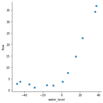
seaborn.lmplot(回归图) 1 2 sns.lmplot('water_level' , 'flow' , data=df, fit_reg=False , size=5 ) plt.show()
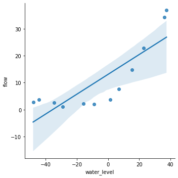
1 2 sns.lmplot('water_level' , 'flow' , data=df, fit_reg=True , size=5 ) plt.show()
1 X, Xval, Xtest = [np.insert(x.reshape(x.shape[0 ], 1 ), 0 , np.ones(x.shape[0 ]), axis=1 ) for x in (X, Xval, Xtest)]
array([[ 1. , -15.93675813],
[ 1. , -29.15297922],
[ 1. , 36.18954863],
[ 1. , 37.49218733],
[ 1. , -48.05882945],
[ 1. , -8.94145794],
[ 1. , 15.30779289],
[ 1. , -34.70626581],
[ 1. , 1.38915437],
[ 1. , -44.38375985],
[ 1. , 7.01350208],
[ 1. , 22.76274892]])代价函数 $$J(\theta)= \frac{1}{2m}\sum_{i=1}^{m}(h_{\theta}(x^{(i)})-y^{(i)})^2$$
1 2 3 4 5 6 7 8 9 10 11 12 13 14 15 16 17 def cost (theta, X, y) : """ X: R(m*n), m records, n features y: R(m) theta : R(n), linear regression parameters """ m = X.shape[0 ] inner = X @ theta - y square_sum = inner.T @ inner cost = square_sum / (2 * m) return cost
1 2 3 4 5 6 7 8 def cost (theta, X, y) : m = X.shape[0 ] inner = X@ theta - y square_sum = inner.T@ inner cost = square_sum / (2 *m) return cost
1 2 3 theta = np.ones(X.shape[1 ]) cost(theta, X, y)
303.95152555359761 2 3 a = np.array([[1 ,3 ],[2 ,4 ]]) b = np.array([[2 ,1 ],[3 ,3 ]]) a @ b
array([[11, 10],
[16, 14]])梯度 $$ \theta_j := \theta_j - \alpha \frac{\partial J(\theta)}{\partial \theta_j}$$
1 2 3 4 5 6 def gradient (theta, X, y) : m = X.shape[0 ] inner = X.T @ (X @ theta - y) return inner / m
array([-15.30301567, 598.16741084])正则化梯度 $$\frac{\partial J(\theta)}{\partial \theta_0} = \frac{1}{m}\sum_{i=1}^{m}(h_{\theta}(x^{(i)})-y^{(i)})x_j^{(i)} ~ for ~j =0$$~ for ~j \geq 1$$
1 2 3 4 5 6 7 8 9 10 def regularized_gradient (theta, X, y, l=1 ) : m = X.shape[0 ] regularized_term = theta.copy() regularized_term[0 ] = 0 regularized_term = (l / m) * regularized_term return gradient(theta, X, y) + regularized_term
1 regularized_gradient(theta, X, y)
array([-15.30301567, 598.25074417])拟合数据
正则化项 $\lambda=0$
1 2 3 4 5 6 7 8 9 10 11 12 13 14 15 16 17 18 19 20 def linear_regression_np (X, y, l=1 ) : """linear regression args: X: feature matrix, (m, n+1) # with incercept x0=1 y: target vector, (m, ) l: lambda constant for regularization return: trained parameters """ theta = np.ones(X.shape[1 ]) res = opt.minimize(fun=regularized_cost, x0=theta, args=(X, y, l), method='TNC' , jac=regularized_gradient, options={'disp' : True }) return res
1 2 3 4 5 6 7 def regularized_cost (theta, X, y, l=1 ) : m = X.shape[0 ] regularized_term = (l / (2 * m)) * np.power(theta[1 :], 2 ).sum() return cost(theta, X, y) + regularized_term
1 2 3 theta = np.ones(X.shape[0 ]) final_theta = linear_regression_np(X, y, l=0 ).get('x' )
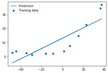
1 2 3 4 5 6 7 b = final_theta[0 ] m = final_theta[1 ] plt.scatter(X[:,1 ], y, label="Training data" ) plt.plot(X[:, 1 ], X[:, 1 ]*m + b, label="Prediction" ) plt.legend(loc=2 ) plt.show()
1 training_cost, cv_cost = [], []
1.使用训练集的子集来拟合应模型
2.在计算训练代价和交叉验证代价时,没有用正则化
3.记住使用相同的训练集子集来计算训练代价
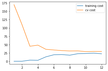
1 2 3 4 5 6 7 8 9 10 11 m = X.shape[0 ] for i in range(1 , m+1 ): res = linear_regression_np(X[:i, :], y[:i], l=0 ) tc = regularized_cost(res.x, X[:i, :], y[:i], l=0 ) cv = regularized_cost(res.x, Xval, yval, l=0 ) training_cost.append(tc) cv_cost.append(cv)
1 2 3 4 plt.plot(np.arange(1 , m+1 ), training_cost, label='training cost' ) plt.plot(np.arange(1 , m+1 ), cv_cost, label='cv cost' ) plt.legend(loc=1 ) plt.show()
这个模型拟合不太好, 欠拟合了
创建多项式特征 1 2 3 4 5 6 7 8 9 10 11 12 13 14 15 16 def prepare_poly_data (*args, power) : """ args: keep feeding in X, Xval, or Xtest will return in the same order """ def prepare (x) : df = poly_features(x, power=power) ndarr = normalize_feature(df).as_matrix() return np.insert(ndarr, 0 , np.ones(ndarr.shape[0 ]), axis=1 ) return [prepare(x) for x in args]
1 2 3 4 5 def poly_features (x, power, as_ndarray=False) : data = {'f{}' .format(i): np.power(x, i) for i in range(1 , power + 1 )} df = pd.DataFrame(data) return df.as_matrix() if as_ndarray else df
1 X, y, Xval, yval, Xtest, ytest = load_data()
1 2 3 data = {'f{}' .format(i): np.power(X, i) for i in range(1 , 3 + 1 )} df = pd.DataFrame(data) df
f1
f2
f3
0
-15.936758
253.980260
-4047.621971
1
-29.152979
849.896197
-24777.006175
2
36.189549
1309.683430
47396.852168
3
37.492187
1405.664111
52701.422173
4
-48.058829
2309.651088
-110999.127750
5
-8.941458
79.949670
-714.866612
6
15.307793
234.328523
3587.052500
7
-34.706266
1204.524887
-41804.560890
8
1.389154
1.929750
2.680720
9
-44.383760
1969.918139
-87432.373590
10
7.013502
49.189211
344.988637
11
22.762749
518.142738
11794.353058
1 2 normalize_feature(df).as_matrix()
c:\users\fishmouse\appdata\local\programs\python\python37\lib\site-packages\ipykernel_launcher.py:1: FutureWarning: Method .as_matrix will be removed in a future version. Use .values instead.
"""Entry point for launching an IPython kernel.
array([[-3.62140776e-01, -7.55086688e-01, 1.82225876e-01],
[-8.03204845e-01, 1.25825266e-03, -2.47936991e-01],
[ 1.37746700e+00, 5.84826715e-01, 1.24976856e+00],
[ 1.42093988e+00, 7.06646754e-01, 1.35984559e+00],
[-1.43414853e+00, 1.85399982e+00, -2.03716308e+00],
[-1.28687086e-01, -9.75968776e-01, 2.51385075e-01],
[ 6.80581552e-01, -7.80028951e-01, 3.40655738e-01],
[-9.88534310e-01, 4.51358004e-01, -6.01281871e-01],
[ 2.16075753e-01, -1.07499276e+00, 2.66275156e-01],
[-1.31150068e+00, 1.42280595e+00, -1.54812094e+00],
[ 4.03776736e-01, -1.01501039e+00, 2.73378511e-01],
[ 9.29375305e-01, -4.19807932e-01, 5.10968368e-01]])1 poly_features(X, power=3 )
f1
f2
f3
0
-15.936758
253.980260
-4047.621971
1
-29.152979
849.896197
-24777.006175
2
36.189549
1309.683430
47396.852168
3
37.492187
1405.664111
52701.422173
4
-48.058829
2309.651088
-110999.127750
5
-8.941458
79.949670
-714.866612
6
15.307793
234.328523
3587.052500
7
-34.706266
1204.524887
-41804.560890
8
1.389154
1.929750
2.680720
9
-44.383760
1969.918139
-87432.373590
10
7.013502
49.189211
344.988637
11
22.762749
518.142738
11794.353058
准备多项式回归数据
扩展特征到 8阶,或者你需要的阶数
使用 归一化 来合并 $x^n$
don’t forget intercept term别忘了截距项
1 2 3 def normalize_feature (df) : """Applies function along input axis(default 0) of DataFrame.""" return df.apply(lambda column: (column - column.mean()) / column.std())
1 2 X_poly, Xval_poly, Xtest_poly= prepare_poly_data(X, Xval, Xtest, power=8 ) X_poly[:3 , :]
array([[ 1.00000000e+00, -3.62140776e-01, -7.55086688e-01,
1.82225876e-01, -7.06189908e-01, 3.06617917e-01,
-5.90877673e-01, 3.44515797e-01, -5.08481165e-01],
[ 1.00000000e+00, -8.03204845e-01, 1.25825266e-03,
-2.47936991e-01, -3.27023420e-01, 9.33963187e-02,
-4.35817606e-01, 2.55416116e-01, -4.48912493e-01],
[ 1.00000000e+00, 1.37746700e+00, 5.84826715e-01,
1.24976856e+00, 2.45311974e-01, 9.78359696e-01,
-1.21556976e-02, 7.56568484e-01, -1.70352114e-01]])画出学习曲线
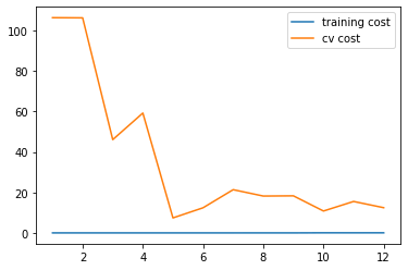
首先,我们没有使用正则化,所以 $\lambda=0$
1 2 3 4 5 6 7 8 9 10 11 12 13 14 15 16 17 18 19 def plot_learning_curve (X, y, Xval, yval, l=0 ) : training_cost, cv_cost = [], [] m = X.shape[0 ] for i in range(1 , m + 1 ): res = linear_regression_np(X[:i, :], y[:i], l=l) tc = cost(res.x, X[:i, :], y[:i]) cv = cost(res.x, Xval, yval) training_cost.append(tc) cv_cost.append(cv) plt.plot(np.arange(1 , m + 1 ), training_cost, label='training cost' ) plt.plot(np.arange(1 , m + 1 ), cv_cost, label='cv cost' ) plt.legend(loc=1 )
1 2 plot_learning_curve(X_poly, y, Xval_poly, yval, l=0 ) plt.show()
你可以看到训练的代价太低了,不真实. 这是 过拟合 了
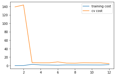
try $\lambda=1$ 1 2 plot_learning_curve(X_poly, y, Xval_poly, yval, l=1 ) plt.show()
训练代价增加了些,不再是0了。过拟合
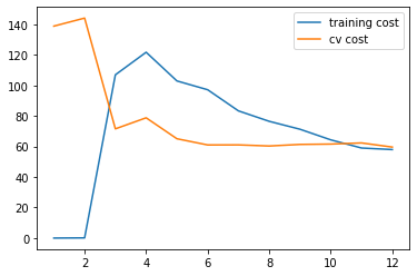
try $\lambda=100$ 1 2 plot_learning_curve(X_poly, y, Xval_poly, yval, l=100 ) plt.show()
太多正则化了.欠拟合 状态
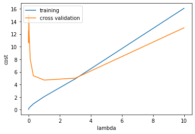
找到最佳的 $\lambda$ 1 2 l_candidate = [0 , 0.001 , 0.003 , 0.01 , 0.03 , 0.1 , 0.3 , 1 , 3 , 10 ] training_cost, cv_cost = [], []
1 2 3 4 5 6 7 8 for l in l_candidate: res = linear_regression_np(X_poly, y, l) tc = cost(res.x, X_poly, y) cv = cost(res.x, Xval_poly, yval) training_cost.append(tc) cv_cost.append(cv)
1 2 3 4 5 6 7 8 plt.plot(l_candidate, training_cost, label='training' ) plt.plot(l_candidate, cv_cost, label='cross validation' ) plt.legend(loc=2 ) plt.xlabel('lambda' ) plt.ylabel('cost' ) plt.show()
1 2 l_candidate[np.argmin(cv_cost)]
11 2 3 4 for l in l_candidate: theta = linear_regression_np(X_poly, y, l).x print('test cost(l={}) = {}' .format(l, cost(theta, Xtest_poly, ytest)))
test cost(l=0) = 10.055426362410126
test cost(l=0.001) = 11.001927632262907
test cost(l=0.003) = 11.26474655167747
test cost(l=0.01) = 10.880780731411715
test cost(l=0.03) = 10.022100517865269
test cost(l=0.1) = 8.63190793331871
test cost(l=0.3) = 7.3366077892272585
test cost(l=1) = 7.466283751156784
test cost(l=3) = 11.643941860536106
test cost(l=10) = 27.715080254176254
调参后, $\lambda = 0.3$ 是最优选择,这个时候测试代价最小
参考链接