本文主要是:通过练习,了解线性回归原理以及 代价函数、梯度下降相关理解
作业内容在根目录: 作业文件
单变量线性回归
1
2
3
import numpy as npimport pandas as pdimport matplotlib.pyplot as plt
1
2
path = 'ex1data1.txt' data = pd.read_csv(path, header=None , names=['Population' , 'Profit' ])
Population
Profit
0
6.1101
17.5920
1
5.5277
9.1302
2
8.5186
13.6620
3
7.0032
11.8540
4
5.8598
6.8233
<bound method DataFrame.info of     Population    Profit
0       6.1101  17.59200
1       5.5277   9.13020
2       8.5186  13.66200
3       7.0032  11.85400
4       5.8598   6.82330
..         ...       ...
92      5.8707   7.20290
93      5.3054   1.98690
94      8.2934   0.14454
95     13.3940   9.05510
96      5.4369   0.61705

[97 rows x 2 columns]>
Population
Profit
count
97.000000
97.000000
mean
8.159800
5.839135
std
3.869884
5.510262
min
5.026900
-2.680700
25%
5.707700
1.986900
50%
6.589400
4.562300
75%
8.578100
7.046700
max
22.203000
24.147000
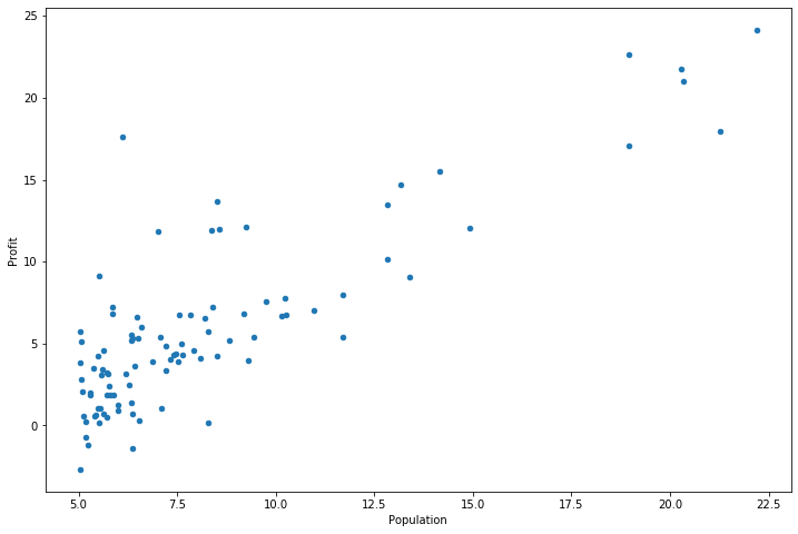
1 2 3 data.plot(kind='scatter' , x='Population' , y='Profit' , figsize=(12 ,8 )) plt.show()
代价函数 现在让我们使用梯度下降来实现线性回归,以最小化成本函数。 以下代码示例中实现的方程在“练习”文件夹中的“ex1.pdf”中有详细说明。
首先,我们将创建一个以参数θ为特征函数的代价函数
1
2
3
def computeCost (X, y, theta) : inner = np.power(((X * theta.T) - y), 2 ) return np.sum(inner) / (2 * len(X))
让我们在训练集中添加一列,以便我们可以使用向量化的解决方案来计算代价和梯度。
1 data.insert(0 , 'Ones' , 1 )
1 data.insert(1 , 'Twos' , 1 )
Ones
Twos
Population
Profit
0
1
1
6.1101
17.59200
1
1
1
5.5277
9.13020
2
1
1
8.5186
13.66200
3
1
1
7.0032
11.85400
4
1
1
5.8598
6.82330
...
...
...
...
...
92
1
1
5.8707
7.20290
93
1
1
5.3054
1.98690
94
1
1
8.2934
0.14454
95
1
1
13.3940
9.05510
96
1
1
5.4369
0.61705
97 rows × 4 columns
删除多添加的列
用法:DataFrame.drop(labels=None,axis=0, index=None, columns=None, inplace=False)
参数说明:
labels 就是要删除的行列的名字,用列表给定
axis 默认为0,指删除行,因此删除columns时要指定axis=1;
index 直接指定要删除的行
columns 直接指定要删除的列
inplace=False,默认该删除操作不改变原数据,而是返回一个执行删除操作后的新dataframe;
inplace=True,则会直接在原数据上进行删除操作,删除后无法返回。
因此,删除行列有两种方式:
1 data.drop(['Twos' ],axis=1 ,inplace=True )
Ones
Population
Profit
0
1
6.1101
17.59200
1
1
5.5277
9.13020
2
1
8.5186
13.66200
3
1
7.0032
11.85400
4
1
5.8598
6.82330
...
...
...
...
92
1
5.8707
7.20290
93
1
5.3054
1.98690
94
1
8.2934
0.14454
95
1
13.3940
9.05510
96
1
5.4369
0.61705
97 rows × 3 columns
1 2 3 4 cols = data.shape[1 ] X = data.iloc[:,0 :cols-1 ] y = data.iloc[:,cols-1 :cols]
观察下 X (训练集) and y (目标变量)是否正确.
Ones
Population
0
1
6.1101
1
1
5.5277
2
1
8.5186
3
1
7.0032
4
1
5.8598
Profit
0
17.5920
1
9.1302
2
13.6620
3
11.8540
4
6.8233
代价函数是应该是numpy矩阵,所以我们需要转换X和Y,然后才能使用它们。 我们还需要初始化theta。
1
2
3
X = np.matrix(X.values) y = np.matrix(y.values) theta = np.matrix(np.array([0 ,0 ]))
matrix([[0, 0]])1 X.shape, theta.shape, y.shape
((97, 2), (1, 2), (97, 1))1 computeCost(X, y, theta)
32.072733877455676batch gradient decent(批量梯度下降) $$ \theta_j:=\theta_j- \alpha \frac{\partial J(\theta)}{\partial \theta_j} $$
1
2
3
4
5
6
7
8
9
10
11
12
13
14
15
16
def gradientDescent (X, y, theta, alpha, iters) : temp = np.matrix(np.zeros(theta.shape)) parameters = int(theta.ravel().shape[1 ]) cost = np.zeros(iters) for i in range(iters): error = (X * theta.T) - y for j in range(parameters): term = np.multiply(error, X[:,j]) temp[0 ,j] = theta[0 ,j] - ((alpha / len(X)) * np.sum(term)) theta = temp cost[i] = computeCost(X, y, theta) return theta, cost
初始化一些附加变量 - 学习速率α和要执行的迭代次数。
1
2
alpha = 0.01 iters = 1000
现在让我们运行梯度下降算法来将我们的参数θ适合于训练集。
1
2
g, cost = gradientDescent(X, y, theta, alpha, iters) g
matrix([[-3.24140214, 1.1272942 ]])
最后,我们可以使用我们拟合的参数计算训练模型的代价函数(误差)。
4.515955503078912
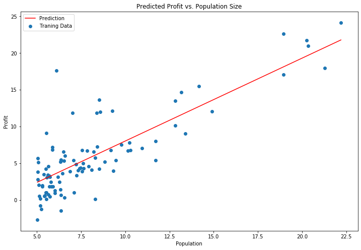
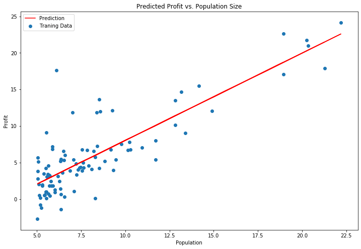
现在我们来绘制线性模型以及数据,直观地看出它的拟合。
1
2
3
4
5
6
7
8
9
10
11
x = np.linspace(data.Population.min(), data.Population.max(), 100 ) f = g[0 , 0 ] + (g[0 , 1 ] * x) fig, ax = plt.subplots(figsize=(12 ,8 )) ax.plot(x, f, 'r' , label='Prediction' ) ax.scatter(data.Population, data.Profit, label='Traning Data' ) ax.legend(loc=2 ) ax.set_xlabel('Population' ) ax.set_ylabel('Profit' ) ax.set_title('Predicted Profit vs. Population Size' ) plt.show()
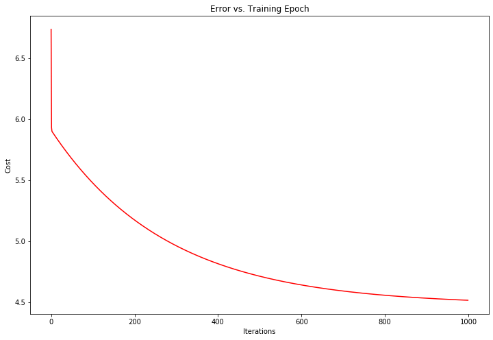
由于梯度方程式函数也在每个训练迭代中输出一个代价的向量,所以我们也可以绘制。 请注意,代价总是降低 - 这是凸优化问题的一个例子。
1
2
3
4
5
6
fig, ax = plt.subplots(figsize=(12 ,8 )) ax.plot(np.arange(iters), cost, 'r' ) ax.set_xlabel('Iterations' ) ax.set_ylabel('Cost' ) ax.set_title('Error vs. Training Epoch' ) plt.show()
多变量线性回归 练习1还包括一个房屋价格数据集,其中有2个变量(房子的大小,卧室的数量)和目标(房子的价格)。 我们使用我们已经应用的技术来分析数据集。
1
2
3
path = 'ex1data2.txt' data2 = pd.read_csv(path, header=None , names=['Size' , 'Bedrooms' , 'Price' ]) data2.head()
Size
Bedrooms
Price
0
2104
3
399900
1
1600
3
329900
2
2400
3
369000
3
1416
2
232000
4
3000
4
539900
对于此任务,我们添加了另一个预处理步骤 - 特征归一化。 这个对于pandas来说很简单
1
2
data2 = (data2 - data2.mean()) / data2.std() data2.head()
Size
Bedrooms
Price
0
0.130010
-0.223675
0.475747
1
-0.504190
-0.223675
-0.084074
2
0.502476
-0.223675
0.228626
3
-0.735723
-1.537767
-0.867025
4
1.257476
1.090417
1.595389
现在我们重复第1部分的预处理步骤,并对新数据集运行线性回归程序。
1 2 3 4 5 6 7 8 9 10 11 12 13 14 15 16 17 18 data2.insert(0 , 'Ones' , 1 ) cols = data2.shape[1 ] X2 = data2.iloc[:,0 :cols-1 ] y2 = data2.iloc[:,cols-1 :cols] X2 = np.matrix(X2.values) y2 = np.matrix(y2.values) theta2 = np.matrix(np.array([0 ,0 ,0 ])) g2, cost2 = gradientDescent(X2, y2, theta2, alpha, iters) computeCost(X2, y2, g2)
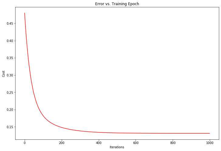
0.1307033696077189我们也可以快速查看这一个的训练进程。
1
2
3
4
5
6
fig, ax = plt.subplots(figsize=(12 ,8 )) ax.plot(np.arange(iters), cost2, 'r' ) ax.set_xlabel('Iterations' ) ax.set_ylabel('Cost' ) ax.set_title('Error vs. Training Epoch' ) plt.show()
我们也可以使用scikit-learn的线性回归函数,而不是从头开始实现这些算法。 我们将scikit-learn的线性回归算法应用于第1部分的数据,并看看它的表现。
1
2
3
from sklearn import linear_modelmodel = linear_model.LinearRegression() model.fit(X, y)
LinearRegression(copy_X=True, fit_intercept=True, n_jobs=None, normalize=False)scikit-learn model的预测表现
1
2
3
4
5
6
7
8
9
10
11
x = np.array(X[:, 1 ].A1) f = model.predict(X).flatten() fig, ax = plt.subplots(figsize=(12 ,8 )) ax.plot(x, f, 'r' , label='Prediction' ) ax.scatter(data.Population, data.Profit, label='Traning Data' ) ax.legend(loc=2 ) ax.set_xlabel('Population' ) ax.set_ylabel('Profit' ) ax.set_title('Predicted Profit vs. Population Size' ) plt.show()
normal equation(正规方程) 正规方程是通过求解下面的方程来找出使得代价函数最小的参数的:$ \frac{\partial J(\theta_j) }{\partial \theta_j}=0 $。
梯度下降与正规方程的比较:
梯度下降:需要选择学习率α,需要多次迭代,当特征数量n大时也能较好适用,适用于各种类型的模型
正规方程:不需要选择学习率α,一次计算得出,需要计算$(X^TX)^{-1}$,如果特征数量n较大则运算代价大,因为矩阵逆的计算时间复杂度为$O(n3)$,通常来说当$n$小于10000 时还是可以接受的,只适用于线性模型,不适合逻辑回归模型等其他模型
1 2 3 4 def normalEqn (X, y) : theta = np.linalg.inv(X.T@X)@X.T@y return theta
1
2
final_theta2=normalEqn(X, y) final_theta2
matrix([[-3.89578088],
[ 1.19303364]])在练习2中,我们将看看分类问题的逻辑回归。