本文主要是：通过学习python处理糖尿病数据集的方法，了解数据集特征，已经线性回归在预测糖尿病中的应用…

实验目的

• 了解糖尿病数据集的基本特征
• 掌握线性回归在预测糖尿病中的应用

实验内容

• 糖尿病数据集（diabetes dataset）基础实验
• 利用糖尿病数据集预测糖尿病实验

实验步骤

实验一：糖尿病数据集基础实验

步骤一：加载数据集

糖尿病（diabetes）数据集，包含在sklearn库的datasets 模块中,调用 load_diabetes 函数来加载数据

1
2
3

from sklearn import datasets
# 加载数据集
diabetes = datasets.load_diabetes()

步骤二：读取糖尿病数据集的描述信息

1
2

# dir()查看diabetes的属性
dir(diabetes)

['DESCR',
 'data',
 'data_filename',
 'feature_names',
 'target',
 'target_filename']

1
2

# diabetes.keys()显示diabetes对象的键，键对应于一定的值
diabetes.keys()

dict_keys(['data', 'target', 'DESCR', 'feature_names', 'data_filename', 'target_filename'])

1
2

# 读取描述信息
print(diabetes.DESCR)

.. _diabetes_dataset:

Diabetes dataset
----------------

Ten baseline variables, age, sex, body mass index, average blood
pressure, and six blood serum measurements were obtained for each of n =
442 diabetes patients, as well as the response of interest, a
quantitative measure of disease progression one year after baseline.

**Data Set Characteristics:**

  :Number of Instances: 442

  :Number of Attributes: First 10 columns are numeric predictive values

  :Target: Column 11 is a quantitative measure of disease progression one year after baseline

  :Attribute Information:
      - Age
      - Sex
      - Body mass index
      - Average blood pressure
      - S1
      - S2
      - S3
      - S4
      - S5
      - S6

Note: Each of these 10 feature variables have been mean centered and scaled by the standard deviation times `n_samples` (i.e. the sum of squares of each column totals 1).

Source URL:
https://www4.stat.ncsu.edu/~boos/var.select/diabetes.html

For more information see:
Bradley Efron, Trevor Hastie, Iain Johnstone and Robert Tibshirani (2004) "Least Angle Regression," Annals of Statistics (with discussion), 407-499.
(https://web.stanford.edu/~hastie/Papers/LARS/LeastAngle_2002.pdf)

步骤三：打印diabetes数据集相关特征信息

1
2
3
4
5
6
7
8
9

# data 、target、统计数据总行数、target长度、每行的属性个数（特征数）、特征名称，数据的类型、data和taret数据集的类型
print("数据：{}\n".format(diabetes.data,'\n'))
print("类标：",diabetes.target,'\n')
print("数据总行数：",len(diabetes.data))
print("类标总长度：",len(diabetes.target))
print("特征数：",len(diabetes.data[0]))
print("特征名称：",diabetes.feature_names)
print("数据类型：",diabetes.data.shape)
print("data类型：",type(diabetes.data),"\n target类型：",type(diabetes.data))

数据：[[ 0.03807591  0.05068012  0.06169621 ... -0.00259226  0.01990842
  -0.01764613]
 [-0.00188202 -0.04464164 -0.05147406 ... -0.03949338 -0.06832974
  -0.09220405]
 [ 0.08529891  0.05068012  0.04445121 ... -0.00259226  0.00286377
  -0.02593034]
 ...
 [ 0.04170844  0.05068012 -0.01590626 ... -0.01107952 -0.04687948
   0.01549073]
 [-0.04547248 -0.04464164  0.03906215 ...  0.02655962  0.04452837
  -0.02593034]
 [-0.04547248 -0.04464164 -0.0730303  ... -0.03949338 -0.00421986
   0.00306441]]

类标： [151.  75. 141. 206. 135.  97. 138.  63. 110. 310. 101.  69. 179. 185.
 118. 171. 166. 144.  97. 168.  68.  49.  68. 245. 184. 202. 137.  85.
 131. 283. 129.  59. 341.  87.  65. 102. 265. 276. 252.  90. 100.  55.
  61.  92. 259.  53. 190. 142.  75. 142. 155. 225.  59. 104. 182. 128.
  52.  37. 170. 170.  61. 144.  52. 128.  71. 163. 150.  97. 160. 178.
  48. 270. 202. 111.  85.  42. 170. 200. 252. 113. 143.  51.  52. 210.
  65. 141.  55. 134.  42. 111.  98. 164.  48.  96.  90. 162. 150. 279.
  92.  83. 128. 102. 302. 198.  95.  53. 134. 144. 232.  81. 104.  59.
 246. 297. 258. 229. 275. 281. 179. 200. 200. 173. 180.  84. 121. 161.
  99. 109. 115. 268. 274. 158. 107.  83. 103. 272.  85. 280. 336. 281.
 118. 317. 235.  60. 174. 259. 178. 128.  96. 126. 288.  88. 292.  71.
 197. 186.  25.  84.  96. 195.  53. 217. 172. 131. 214.  59.  70. 220.
 268. 152.  47.  74. 295. 101. 151. 127. 237. 225.  81. 151. 107.  64.
 138. 185. 265. 101. 137. 143. 141.  79. 292. 178.  91. 116.  86. 122.
  72. 129. 142.  90. 158.  39. 196. 222. 277.  99. 196. 202. 155.  77.
 191.  70.  73.  49.  65. 263. 248. 296. 214. 185.  78.  93. 252. 150.
  77. 208.  77. 108. 160.  53. 220. 154. 259.  90. 246. 124.  67.  72.
 257. 262. 275. 177.  71.  47. 187. 125.  78.  51. 258. 215. 303. 243.
  91. 150. 310. 153. 346.  63.  89.  50.  39. 103. 308. 116. 145.  74.
  45. 115. 264.  87. 202. 127. 182. 241.  66.  94. 283.  64. 102. 200.
 265.  94. 230. 181. 156. 233.  60. 219.  80.  68. 332. 248.  84. 200.
  55.  85.  89.  31. 129.  83. 275.  65. 198. 236. 253. 124.  44. 172.
 114. 142. 109. 180. 144. 163. 147.  97. 220. 190. 109. 191. 122. 230.
 242. 248. 249. 192. 131. 237.  78. 135. 244. 199. 270. 164.  72.  96.
 306.  91. 214.  95. 216. 263. 178. 113. 200. 139. 139.  88. 148.  88.
 243.  71.  77. 109. 272.  60.  54. 221.  90. 311. 281. 182. 321.  58.
 262. 206. 233. 242. 123. 167.  63. 197.  71. 168. 140. 217. 121. 235.
 245.  40.  52. 104. 132.  88.  69. 219.  72. 201. 110.  51. 277.  63.
 118.  69. 273. 258.  43. 198. 242. 232. 175.  93. 168. 275. 293. 281.
  72. 140. 189. 181. 209. 136. 261. 113. 131. 174. 257.  55.  84.  42.
 146. 212. 233.  91. 111. 152. 120.  67. 310.  94. 183.  66. 173.  72.
  49.  64.  48. 178. 104. 132. 220.  57.] 

数据总行数： 442
类标总长度： 442
特征数： 10
特征名称： ['age', 'sex', 'bmi', 'bp', 's1', 's2', 's3', 's4', 's5', 's6']
数据类型： (442, 10)
data类型： <class 'numpy.ndarray'> 
 target类型： <class 'numpy.ndarray'>

实验二：利用糖尿病数据集预测糖尿病实验

步骤一：LinearRegression（线性回归）的引用

• LinearRegression模型在Sklearn.linear_model下，它主要是通过fit(x,y)的方法来训练模型，其中x为数据的属性，y为所属类型。
• 线性模型：$$y = βX+b$$
  其中：(X:数据 y：目标变量 β：回归系数 b:观测噪声（bias，偏差)

• 引用回归模型，并输出函数原型

1
2
3
4

# 引用回归模型
from sklearn import linear_model # 导入线性回归模型
regr = linear_model.LinearRegression()# 使用线性回归
print(regr) #输出函数原型

LinearRegression(copy_X=True, fit_intercept=True, n_jobs=None, normalize=False)

• 查看线性回归对象regr的属性和方法

1

dir(regr)

['__abstractmethods__',
 '__class__',
 '__delattr__',
 '__dict__',
 '__dir__',
 '__doc__',
 '__eq__',
 '__format__',
 '__ge__',
 '__getattribute__',
 '__getstate__',
 '__gt__',
 '__hash__',
 '__init__',
 '__init_subclass__',
 '__le__',
 '__lt__',
 '__module__',
 '__ne__',
 '__new__',
 '__reduce__',
 '__reduce_ex__',
 '__repr__',
 '__setattr__',
 '__setstate__',
 '__sizeof__',
 '__str__',
 '__subclasshook__',
 '__weakref__',
 '_abc_impl',
 '_decision_function',
 '_estimator_type',
 '_get_param_names',
 '_get_tags',
 '_more_tags',
 '_preprocess_data',
 '_set_intercept',
 'copy_X',
 'fit',
 'fit_intercept',
 'get_params',
 'n_jobs',
 'normalize',
 'predict',
 'score',
 'set_params']

步骤二：训练和预测方法基础

• 训练：fit(x,y)
  
  分析模型参数，填充数据集。其中x为特征，y为标记或类属性。
• 预测： predict()
  
  它通过fit()算出的模型参数构成的模型，对解释变量进行预测其类属性。预测方法将返回预测值y_pred。

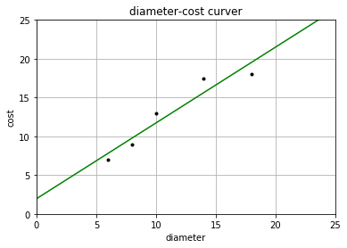
步骤三：利用线性回归的示例

1
2
3
4
5
6
7
8
9
10
11
12
13
14
15
16
17

from sklearn import linear_model # 导入线性模型
import matplotlib.pyplot as plt # 绘图
import numpy as np

# X 表示匹萨尺寸 Y表示匹萨价格
X =[[6],[8],[10],[14],[18]]
Y = [[7],[9],[13],[17.5],[18]]

print(u'数据集X:',X)
print(u'数据集Y:',Y)
# 回归训练
clf2 = linear_model.LinearRegression() # 使用线性回归
clf2.fit(X,Y) # 导入数据集

# 预测一张12英寸的价格
res = clf2.predict(np.array([12]).reshape(1,1))[0]
print(u'预测一张12英寸的匹萨价格：$%.2f'%res)

数据集X: [[6], [8], [10], [14], [18]]
数据集Y: [[7], [9], [13], [17.5], [18]]
预测一张12英寸的匹萨价格：$13.68

• 请解释np.array([12]).reshape(1,1)及字符串前加u的意义

1

#

• 预测数据X2 = [[0],[10],[14],[25]]的结果

1
2
3
4

# 预测数据X2 = [[0],[10],[14],[25]]
X2 = [[0],[10],[14],[25]]
Y2 = clf2.predict(X2)
print(Y2)

[[ 1.96551724]
 [11.72844828]
 [15.63362069]
 [26.37284483]]

• 绘制线性回归图形

1
2
3
4
5
6
7
8
9

plt.figure()
plt.title(u'diameter-cost curver') #标题
plt.xlabel(u'diameter') #x轴坐标
plt.ylabel(u'cost')   # y轴
plt.axis([0,25,0,25]) #区间
plt.grid(True) # 显示网格
plt.plot(X,Y,'k.') #绘制训练数据集散点图
plt.plot(X2,Y2,'g-')# 绘制预测数据集直线
plt.show()

• 线性模型：$$y = βX+b$$
  其中回归系数β保存在coef_方法中，截距保存在intercept_中，
  score(X,y,sample_weight=None) 评分函数，返回一个小于1的得分，可能会小于0

1
2
3
4

#打印系数、截距、评分函数
print(u'系数',clf2.coef_)
print(u'截距',clf2.intercept_)
print(u'评分函数',clf2.score(X,Y))

系数 [[0.9762931]]
截距 [1.96551724]
评分函数 0.9100015964240102

步骤四：糖尿病数据集划分

• 加载diabetes数据集,并打印数据集长度、数据类型、前四个样本数据

1
2
3
4
5
6
7

from sklearn import datasets
import numpy as np

# 获取数据 10*442
d =datasets.load_diabetes()
x = d.data
print(u'获取x特征',len(x),x.shape,x[:4])

获取x特征 442 (442, 10) [[ 0.03807591  0.05068012  0.06169621  0.02187235 -0.0442235  -0.03482076
  -0.04340085 -0.00259226  0.01990842 -0.01764613]
 [-0.00188202 -0.04464164 -0.05147406 -0.02632783 -0.00844872 -0.01916334
   0.07441156 -0.03949338 -0.06832974 -0.09220405]
 [ 0.08529891  0.05068012  0.04445121 -0.00567061 -0.04559945 -0.03419447
  -0.03235593 -0.00259226  0.00286377 -0.02593034]
 [-0.08906294 -0.04464164 -0.01159501 -0.03665645  0.01219057  0.02499059
  -0.03603757  0.03430886  0.02269202 -0.00936191]]

• 获取第3列体重特征的数据,并打印前四行的数据

1
2

x_one = x[:,np.newaxis,2]
print(x_one[:4])

[[ 0.06169621]
 [-0.05147406]
 [ 0.04445121]
 [-0.01159501]]

• 获取类标target,并打印前四个

1
2

y = d.target
print(u'target:',y[:4])

target: [151.  75. 141. 206.]

• x特征划分：训练集和测试集；后42行作为测试集，剩余的作为训练集

1
2
3
4
5
6
7

#训练集
x_train = x_one[:-42]
y_train = y[:-42]

# 测试集
x_test = x_one[-42:]
y_test = y[-42:]

步骤五:糖尿病的线性回归实现

1
2
3
4
5
6
7
8

from sklearn import linear_model
clf = linear_model.LinearRegression()
# 训练
clf.fit(x_train,y_train)
#预测
pre = clf.predict(x_test)
print(u'预测结果：{}\n'.format(pre))
print(u'真实结果：',y_test)

预测结果：[196.51241167 109.98667708 121.31742804 245.95568858 204.75295782
 270.67732703  75.99442421 241.8354155  104.83633574 141.91879342
 126.46776938 208.8732309  234.62493762 152.21947611 159.42995399
 161.49009053 229.47459628 221.23405012 129.55797419 100.71606266
 118.22722323 168.70056841 227.41445974 115.13701842 163.55022706
 114.10695016 120.28735977 158.39988572 237.71514243 121.31742804
  98.65592612 123.37756458 205.78302609  95.56572131 154.27961264
 130.58804246  82.17483382 171.79077322 137.79852034 137.79852034
 190.33200206  83.20490209]

真实结果： [175.  93. 168. 275. 293. 281.  72. 140. 189. 181. 209. 136. 261. 113.
 131. 174. 257.  55.  84.  42. 146. 212. 233.  91. 111. 152. 120.  67.
 310.  94. 183.  66. 173.  72.  49.  64.  48. 178. 104. 132. 220.  57.]

步骤六:对上述预测结果进行评价

• 分别从预测结果和真实结果之间的平方和、线性回归模型的系数、截距、方差

1
2
3
4
5

cost = np.mean(y_test-pre)**2
print('平方和：{}\n'.format(cost))
print('系数：{}\n'.format(clf.coef_))
print('截距：{}\n'.format(clf.intercept_))
print('决定系数：{}\n'.format(clf.score(x_test,y_test)))

平方和：83.19234082703763

系数：[955.70303385]

截距：153.00018395675963

决定系数：0.42720426706720194

​

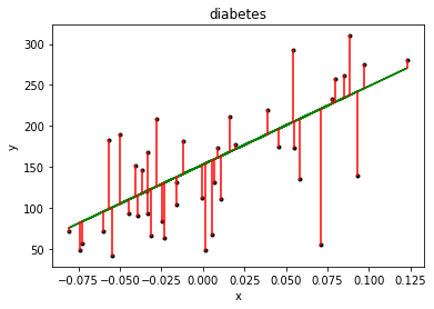
步骤七:绘图

• 分别绘制出测试集的真实散点图，预测的线性图，以及画出各个真实点到预测点的距离，并保存到diabetes.png中，dpi=300

1
2
3
4
5
6
7
8
9
10
11
12
13

import matplotlib.pyplot as plt
plt.title('diabetes')
plt.xlabel('x')
plt.ylabel('y')
plt.plot(x_test,y_test,'k.')# 测试集真实散点图
plt.plot(x_test,pre,'g-')# 预测线性直线

# 绘制真实点到预测点的线段
for idx ,m in enumerate(x_test):
    plt.plot([m,m],[y_test[idx],pre[idx]],'r-')
    
plt.savefig('diabetes.png',dpi=300)
plt.show()