【数据集分析】新冠肺炎COVID-19数据集简单分析与处理

本文主要是：新冠肺炎COVID-19 State Data Set的简单分析与处理

Step 1

Use Pandas to load COVID-19 State Data Set as the dataframe.
Pandas

由于数据持续更新,所以下载链接仅供参考，链接：https://pan.baidu.com/s/1npzHaEX5DUudB1yTTm8hyQ
提取码：qy8i

若需要请到此，下载最新数据COVID-19 State Data Set

1
2
3
4

import pandas as pd
data = pd.read_csv('COVID19_state.csv')
df = pd.DataFrame(data)
df

1

df.keys()

Index(['State', 'Tested', 'Infected', 'Deaths', 'Population', 'Pop Density',
       'Gini', 'ICU Beds', 'Income', 'GDP', 'Unemployment', 'Sex Ratio',
       'Smoking Rate', 'Flu Deaths', 'Respiratory Deaths', 'Physicians',
       'Hospitals', 'Health Spending', 'Pollution', 'Med-Large Airports',
       'Temperature', 'Urban', 'Age 0-25', 'Age 26-54', 'Age 55+',
       'School Closure Date'],
      dtype='object')

Step 2

Get 20 data items as sample randomly and show them.

1
2

df1 = df.sample(frac=0.4)
df1

Step 3

Show 10 data items which the Deaths are more than 100 as sample randomly.

1
2
3

df2 = df[df['Deaths']>100]
df3 = df2.sample(n = 10)
df3

Step 4

Sort the data by GDP and present the top 20 data items.

1
2

df4= df.sort_values(by=['GDP'])
df4.iloc[0:20,]

Step 5

Show the simple statistical information (mean, std, min, max, quartile1, quartile2, quartile3).

1
2
3

#1.mean
print(df.mean())# 列平均
print(df.mean(1))# 行平均

1
2
3

# 2.std
print(df.std()) # 列std
print(df.std(1))

1
2

# 3.min
print(df.min())

1
2

# 4.df.min()
df.max()

1
2

# 5.quartile1
df.quantile()

1
2

# 6.
df.quantile(q=0.5)

1
2

# 7.
df.quantile(q=0.75)

Step 6

Use matplotlib show 2D images about data.

Matplotlib

Plot the distribution of two class (1. GDP < 58000, 2. GDP >= 58000) of COVID-19 State Data using different colors and different marker where x-axis is the Pollution and y-axis the Mortality-rate.

1
2
3
4
5
6
7
8
9
10
11

import matplotlib.pyplot as plt

df_GDP1 = df[df['GDP']<58000]
df_GDP2 = df[df['GDP']>=58000]
plt.figure()
ax1 = df_GDP1.plot(x='Pollution',y='Deaths')
df_GDP2.plot(x='Pollution',y='Deaths',ax=ax1)
# 为图表添加标题
plt.title("testddddd")

plt.show()

<Figure size 432x288 with 0 Axes>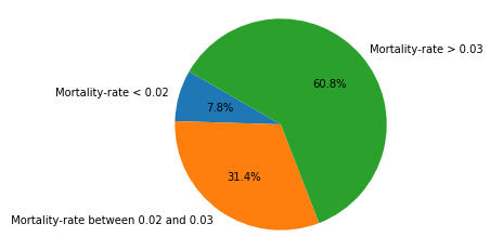

Step 7

Show the proportion of three class of COVID-19 State Data using pie chart.

About the class:

1、 Mortality-rate < 0.02

2、 Mortality-rate between 0.02 and 0.03

3、Mortality-rate > 0.03

1
2
3
4
5
6
7
8
9
10
11
12
13
14
15
16
17
18

# 死亡率<0.02
sizes= []
df_death1 = df[df['Deaths']/df['Infected']<0.02]
d1= df_death1.shape[0]  # 返回行数
sizes.append(d1)
# 死亡率在0.02 and 0.03之间
df_death2 = df[df['Deaths']/df['Infected']<=0.03]
d2 = df_death2.shape[0] - d1
sizes.append(d2)
# 死亡率在0.03之上
df_death3 = df[df['Deaths']/df['Infected']>0.03]
d3 = df_death3.shape[0]
sizes.append(d3)

labels = ['Mortality-rate < 0.02',' Mortality-rate between 0.02 and 0.03','Mortality-rate > 0.03']
plt.pie(sizes,labels=labels,autopct='%1.1f%%',shadow=False,startangle=150)
plt.axis('equal')   #该行代码使饼图长宽相等
plt.show()

参考链接

• 饼图绘制：
  • https://www.cnblogs.com/biyoulin/p/9565350.html
  • https://www.jianshu.com/p/0a76c94e9db7
  • https://blog.csdn.net/ChenVast/article/details/81632794
• Panda DataFrame 绘图
  • https://blog.csdn.net/weixin_39778570/article/details/81143763
• Pandas数据帧（DataFrame）
  • https://www.yiibai.com/pandas/python_pandas_dataframe.html
  • https://www.cnblogs.com/dev-liu/p/pandas_plt_basic.html
  • https://blog.csdn.net/zhengxu25689/article/details/87347700
• 其他
  https://blog.csdn.net/kylinxjd/article/details/98307811